Chapter 1: Introduction
- §1. Line Elements
- §2. Circle Trig
- §3. Hyperbola Trig
- §4. Geometry of SR
- §5. Differential Forms
- §6. Geodesics
- §7. The Physics of GR
Line Elements
The fundamental notion in geometry is distance. One can study shapes without worrying about size or scale, but that is topology; in geometry, size matters.
So how do you measure distance? With a ruler. But how do you calibrate the ruler?

In Euclidean geometry, these questions are answered by the Pythagorean Theorem. In infinitesimal form, 1) and in standard rectangular coordinates, the Pythagorean Theorem tells us that \begin{equation} ds^2 = dx^2 + dy^2 \label{R2} \end{equation} as shown in Figure 1. This version of the Pythagorean Theorem not only tells us about right triangles, but also how to measure length along any curve: Just integrate (the square root of) this expression to determine the arclength.
More generally, an expression such as ($\ref{R2}$) is called a line element, and is also often referred to as the metric tensor, or simply as the metric.
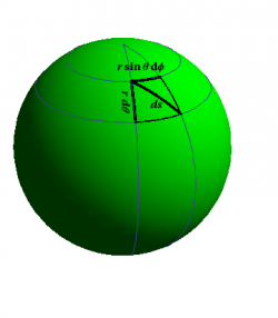
The line element ($\ref{R2}$) describes a Euclidean plane, which is flat. What is the line element for a sphere? That's easy: Draw a picture! Figure 2 shows two “nearby” points on the sphere, separated by a distance $ds$, broken up into pieces of lengths $r\,d\theta$ at constant longitude and $r\,\sin\theta\,d\phi$ at constant latitude. 2) Alternatively, write down the line element for three-dimensional Euclidean space in rectangular coordinates, convert everything to spherical coordinates, then hold $r$ constant. Yes, the algebra is messy. The resulting line element is \begin{equation} ds^2 = r^2 \left( d\theta^2 + \sin^2\theta\,d\phi^2 \right) \label{S2} \end{equation} The study of such curved objects is called Riemannian geometry.
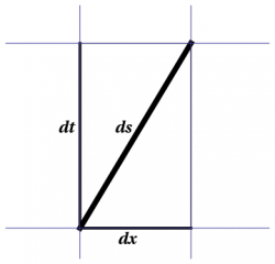
Both line elements above are positive definite, but we can also study geometries which do not have this property. The simplest example is \begin{equation} ds^2 = dx^2 - dt^2 \label{SR} \end{equation} which turns out to describe special relativity; this geometry turns out to be flat, and is called Minkowskian. We classify line elements by their signature $s$, which counts the number of minus signs; $s=1$ for both special and general relativity. Figure 3 shows the infinitesimal Pythagorean Theorem for Minkowski space (special relativity). Yes, this figure looks the same as Figure 1, but this geometry is not that of an ordinary piece of paper. We use this representation because Minkowski space turns out to be flat, but the minus sign in the Pythagorean Theorem leads to a counterintuitive notion of “distance”.
Finally, we can combine the lack of positive-definiteness with curvature; such geometries are called Lorentzian, and describe general relativity. We will study several of these geometries in subsequent chapters.
The different types of geometries referred to above are summarized in Table 1 below. But what does signature mean? In relativity, both special and general, we distinguish between spacelike intervals, for which $ds^2>0$, timelike intervals, for which $ds^2<0$, and lightlike (or null) intervals, for which $ds^2=0$. For spacelike intervals, $ds$ measures the distance between nearby points (along a given path). For timelike intervals, \begin{equation} d\tau = \sqrt{-ds^2} \end{equation} measures the time between nearby points (along a given trajectory). The parameter $\tau$ is often referred to as proper time, generalizing the familiar interpretation of $s$ as arclength.
We begin our exploration of these geometries with a review of trigonometry.
| s=0 | s=1 | |
|---|---|---|
| flat | Euclidean | Minkowskian |
| curved | Riemannian | Lorentzian |
Table 1: Classification of geometries by curvature and signature.
1)
We work throughout with infinitesimal quantities such as $dx$, which can be
thought of informally as “very small”, or more formally as differential
forms, a special kind of tensor. Some further discussion can be found
in §Differentials.
2)
We use “physics” conventions, with $\theta$ measuring colatitude and $\phi$
measuring longitude, and we measure both “sides” of our right
“triangle” starting at the same point, as is appropriate for infinitesimal
objects in curvilinear coordinates. For further details, see our
online vector calculus text.